Stock Price

Thanks my teammates: XIAOLEI (JADEN) CHENG, YANAN (LANCE) LU, YUQI (MARTIN) ZHAI, AND ZEQI (GEORGE) WANG

Introduction

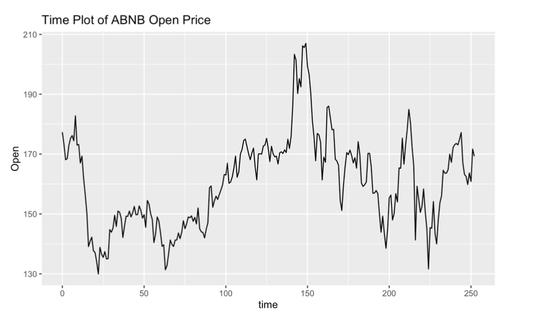
Stock price modeling and prediction is always a critical topic in financial and statistical analysis. However, the stock price is prone to uncertainty and volatility, making it difficult to be accurately predicted. Time series analysis allows us to analyze constantly changing time series data in order to extract meaningful characteristics of the data and forecast short-term future values. This project aims to use conventional time series analysis to forecast the t+1 stock price for Airbnb, Inc. (ABNB) based on its one year historical data during the period April 19, 2021 to April 19, 2022, with 253 trading days in total. The data was collected from Yahoo! Finance on April 20, 2022, where we focus on the opening price as the main interest of this project. The problem we want to explore is how its stock price will change after the surge in COVID19 in early 2022.

Variance Stabilizing Transformation

We use the Box-Cox transformation to pursue homoscedasticity of the original model. As shown on the likelihood plot below, we test the performance of different parameters. -0.788 returns the highest log-likelihood, so we choose -0.788 to be our Box-Cox transformation parameter.

Parametric Model

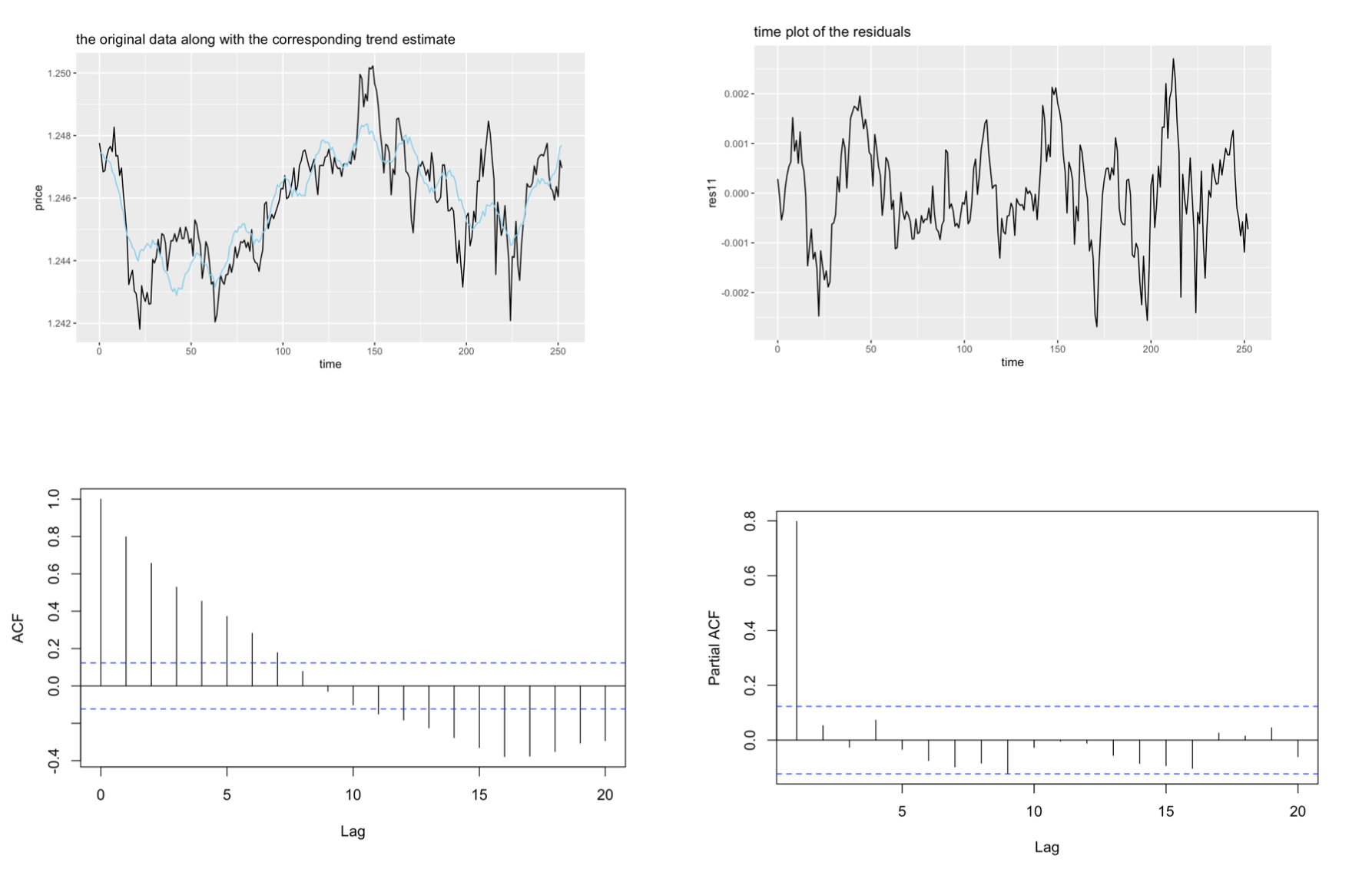
After the variance stabilizing transformation, we use a parametric polynomial and a sinusoidal function to capture the signal.In this parametric model, we include t from power 1 to 5 to model the trend and include the sine and cosine component to model the seasonality as well as the indicators for each weekday. The frequency index 11 is chosen from the periodogram after we fit the model with other features. The reason for not selecting additional frequencies is to avoid potential overfitting.

Noise AR(1)

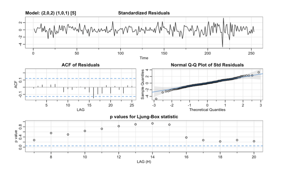
Noise SARIMA(2,0,2)(1,0,1)[5]

Fourth Order Differencing by Lag 1

After applying a parametric model, we decide to use differencing, a non-parametric signal model, to pursue stationarity. We find that there are 3 changes in concavity in the data plot, namely around day 50, 150, and 225, therefore we are inclined to conclude that there must be at least a fourth order polynomial to capture these 3 changes in concavity. Thus, this model performs differencing by lag 1 for 4 times

Looking at the graph after fourth order differencing, we can safely tell that the residual plot is more likely to be a stationary process except a huge oscillation from day 200 to day 230, which can be explained by the come-back of COVID-19 in the beginning of 2022. Seasonality may not be clear in this dataset, since the R builtin function “findfrequency” has a return value 1, which indicates that there is no clear seasonality exhibited in the data provided.

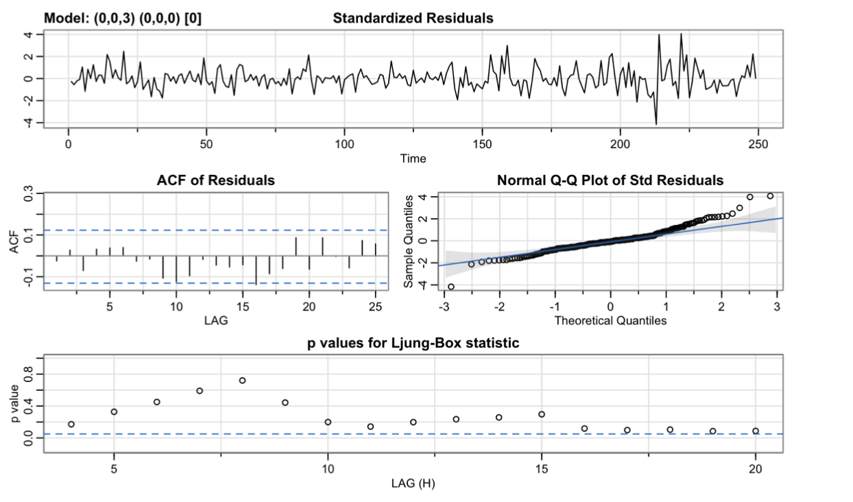
Noise MA(3)

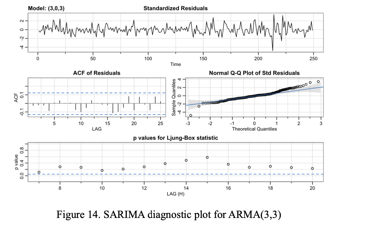
Noise ARMA(3,3)

Model Comparison and Selection

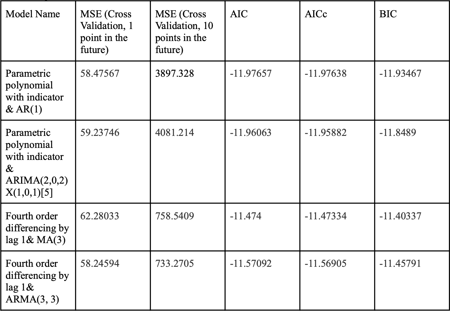
The criteria that we used here includes both in-sample information criterion and out-sample score from cross validation. Judging from the scores shown in Table 1, we can see that for in-sample criteria, model 1 (parametric model with indicator and AR(1)) has the lowest AIC, BIC, and AICc, which means if we are only interested in in-sample fit, the very first model is the most desirable out of all the other models. For out-sample criterion, it is obvious that our fourth model (fourth order differencing with ARMA(3,3)) has the lowest mean squared error for both predicting one point per iteration (disregarding the cascading effect in prediction) and 10 points per iteration (taking into consideration the cascading effect in prediction) in cross validation. Taking into account the ultimate goal for this model is to predict future (t+1 to t+10) opening prices for Airbnb stock prices, we will favor the model with the lowest mean squared error in cross-validation, meaning the lowest out-sample error, better predicting the future value. Therefore, our model selection for this project is the last model, fourth order differencing with ARMA(3,3).

Estimation of model parameters

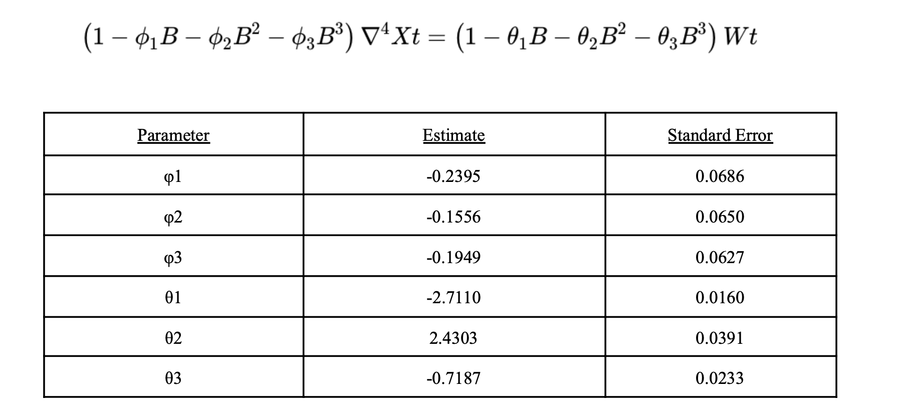
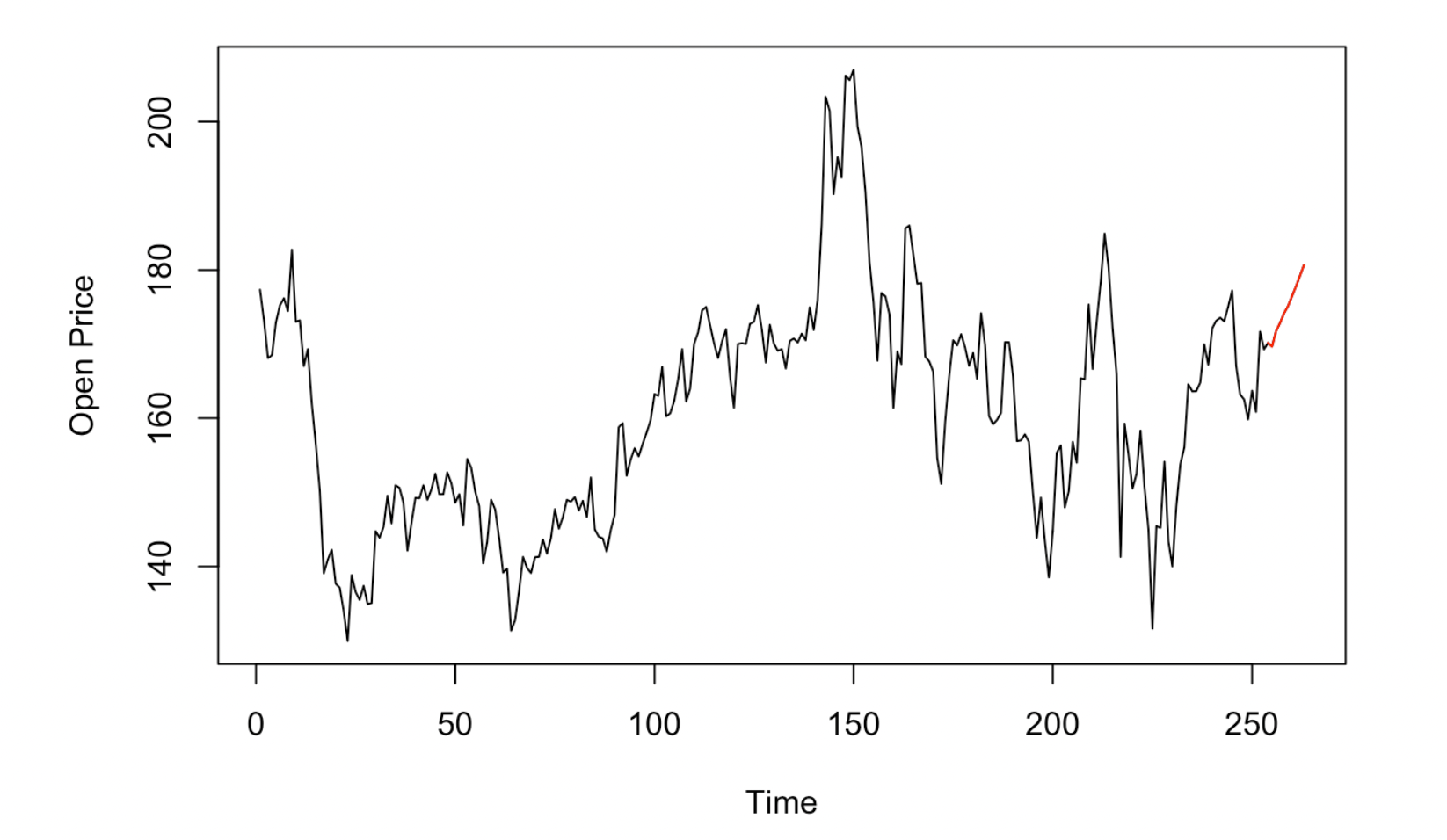
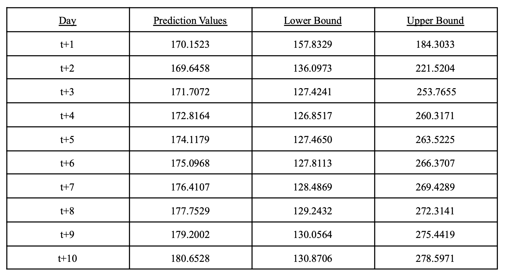
According to the results, the red line segment at the end of figure 15 represents the predictions from model4 that we trained. This overall trend makes sense in the real-life because with the COVID threat passes, the amount of people willing to travel and live in Airbnb will increase, which is reflected in the prediction that we came up with. We also addressed the uncertainty in the parameters and also generated the predictions for the 95% confidence interval from changing the parameters in the ARMA model with an interval of 1.96 * standard error. This confidence interval is not included in the graph but we printed out the predictions and included below in the table.

Prediction